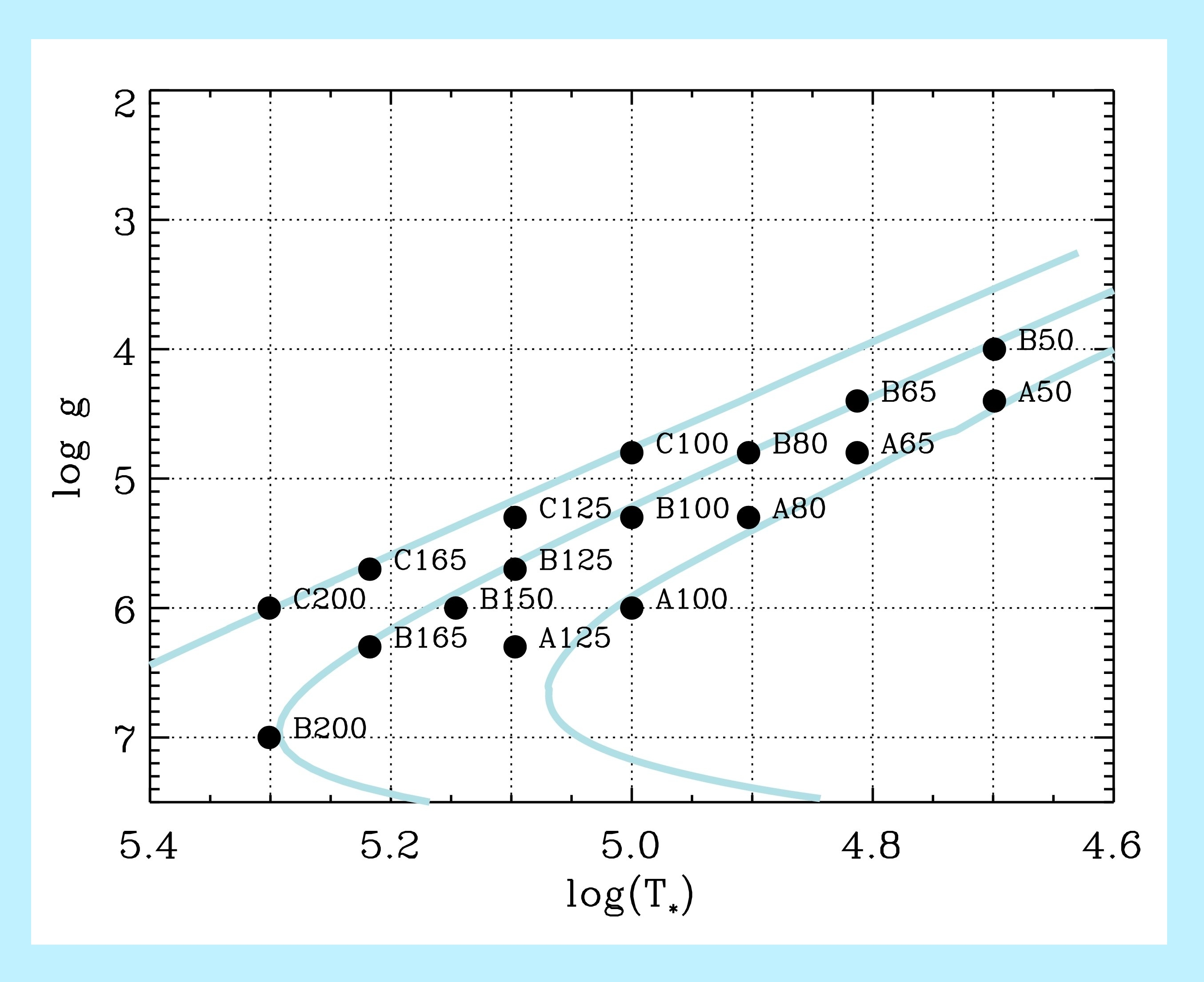
Fig. 1 Grid points in the logT∗-logg
plane. The
evolutionary tracks of Miller Bertolami and Althaus (2006) are also
shown (continuous lines) for CSPNe with 0.5, 0.6, and 0.9 M⊙,
from
right
to
left.
Each point shown in figure 1 is identified by a label which
corresponds to a group of models with approximately the same
temperature, surface
gravity, and radius, but with a range of mass-loss rates and terminal
wind velocities, as can be seen in the tables below. There, the models
are identified by approximated values of the parameters. Precise values
are available at each model page, accessible through the links in the
tables, along with the calculated detailed spectrum (900 - 50000Å) and
continuum (which covers the whole range of wavelength where the flux is
above ~5x10⁻⁴ Jy and includes some dieletronic lines). The
spectrum and
continuum files are named obs_fin and obs_cont, respectively, according
to the nomenclature used by CMFGEN (Hillier and Miller 1998). The files
contain a list of frequencies (in 1015 Hz) and then list the
corresponding fluxes in Janskies assuming a distance of 1kpc. Tables
listing the ions included in the calculations of each model and the
number of levels and superlevels adopted are also available in the
links within the tables below.
Track A
The following table lists the models
that belong to the evolutionary track for CSPNe with 0.5 M⊙,
which
we
refer
to
as
track
A.
Information about the models and the calculated
spectra can be
accessed trough the links in the table. Plots comparing different
models are available at the 'preview' links.
| Model | T∗(kK) | logg | R∗(R☉) | L∗(103L☉) | logṀ(M☉/yr) | v∞(km/s) | Rt(R☉) |
| A50.M73.V500 | 50 | 4.4 | 0.75 | 3.10 | -7.30 | 500 | 40.3 |
| A50.M73.V1000 preview | " | " | " | " | " | 1000 | 64.0 |
| A50.M67.V500 | " | " | " | " | -6.70 | 500 | 16.0 |
| A50.M67.V1000 preview | " | " | " | " | " | 1000 | 25.4 |
| A50.M63.V500 | " | " | " | " | -6.30 | 500 | 8.7 |
| A50.M63.V1000 preview | " | " | " | " | " | 1000 | 13.8 |
| A65.M73.V500 | 65 | 4.8 | 0.47 | 3.50 | -7.30 | 500 | 25.6 |
| A65.M73.V1000 preview | " | " | " | " | " | 1000 | 40.6 |
| A65.M67.V500 | " | " | " | " | -6.70 | 500 | 10.1 |
| A65.M67.V1000 preview | " | " | " | " | " | 1000 | 16.1 |
| A65.M63.V500 | " | " | " | " | -6.30 | 500 | 5.5 |
| A65.M63.V1000 preview | " | " | " | " | " | 1000 | 8.7 |
| A80.M73.V500 | 80 | 5.3 | 0.27 | 2.50 | -7.30 | 500 | 14.4 |
| A80.M73.V1000 preview | " | " | " | " | " | 1000 | 22.8 |
| A80.M67.V500 | " | " | " | " | -6.70 | 500 | 5.7 |
| A80.M67.V1000 preview | " | " | " | " | " | 1000 | 9.0 |
| A80.M63.V500 | " | " | " | " | -6.30 | 500 | 3.1 |
| A80.M63.V1000 preview | " | " | " | " | " | 1000 | 4.9 |
| A100.M73.V1500 | 100.00 | 6.0 | 0.12 | 1.20 | -7.30 | 1500 | 13.3 |
| A100.M73.V2000 preview | " | " | " | " | " | 2000 | 16.1 |
| A100.M73.V2500 | " | " | " | " | " | 2500 | 18.7 |
| A100.M70.V1500 | " | " | " | " | -7.00 | 1500 | 8.4 |
| A100.M70.V2000 preview | " | " | " | " | " | 2000 | 10.2 |
| A100.M70.V2500 | " | " | " | " | " | 2500 | 11.8 |
| A100.M67.V1500 | " | " | " | " | -6.70 | 1500 | 5.3 |
| A100.M67.V2000 preview | " | " | " | " | " | 2000 | 6.4 |
| A100.M67.V2500 | " | " | " | " | " | 2500 | 7.4 |
| A125.M73.V1500 | 125 | 6.3 | 0.08 | 1.50 | -7.30 | 1500 | 9.4 |
| A125.M73.V2000 preview | " | " | " | " | " | 2000 | 11.4 |
| A125.M73.V2500 | " | " | " | " | " | 2500 | 13.3 |
| A125.M70.V1500 | " | " | " | " | -7.00 | 1500 | 5.9 |
| A125.M70.V2000 preview | " | " | " | " | " | 2000 | 7.2 |
| A125.M70.V2500 | " | " | " | " | " | 2500 | 8.4 |
| A125.M67.V1500 | " | " | " | " | -6.70 | 1500 | 3.7 |
| A125.M67.V2000 preview | " | " | " | " | " | 2000 | 4.5 |
| A125.M67.V2500 | " | " | " | " | " | 2500 | 5.3 |
Track B
The following table lists the models that belong to the evolutionary track for CSPNe with 0.6 M⊙, which we refer to as track B. Information about the models and the calculated spectra can be accessed trough the links in the table. Plots comparing different models are available at the 'preview' links.
| Model | T∗(kK) | logg | R∗(R☉) | L∗(103L☉) | logṀ(M☉/yr) | v∞(km/s) | Rt(R☉) |
| B50.M70.V500 | 50 | 4.0 | 1.29 | 9.20 | -7.00 | 500 | 43.8 |
| B50.M70.V1000 ab preview | " | " | " | " | " | 1000 | 69.5 |
| B50.M63.V500 | " | " | " | " | -6.30 | 500 | 15.0 |
| B50.M63.V1000 ab preview | " | " | " | " | " | 1000 | 23.8 |
| B50.M60.V500 | " | " | " | " | -6.00 | 500 | 9.4 |
| B50.M60.V1000 ab preview | " | " | " | " | " | 1000 | 15.0 |
| B65.M70.V500 | 65 | 4.4 | 0.82 | 10.50 | -7.00 | 500 | 27.9 |
| B65.M70.V1000 ab preview | " | " | " | " | " | 1000 | 44.2 |
| B65.M63.V500 | " | " | " | " | -6.30 | 500 | 9.5 |
| B65.M63.V1000 ab preview | " | " | " | " | " | 1000 | 15.1 |
| B65.M60.V500 | " | " | " | " | -6.00 | 500 | 6.0 |
| B65.M60.V1000 ab preview | " | " | " | " | " | 1000 | 9.5 |
| B80.M70.V500 | 80 | 4.8 | 0.52 | 9.60 | -7.00 | 500 | 17.6 |
| B80.M70.V1000 ab preview | " | " | " | " | " | 1000 | 27.9 |
| B80.M63.V500 | " | " | " | " | -6.30 | 500 | 6.0 |
| B80.M63.V1000 ab preview | " | " | " | " | " | 1000 | 9.5 |
| B80.M60.V500 | " | " | " | " | -6.00 | 500 | 3.8 |
| B80.M60.V1000 ab preview | " | " | " | " | " | 1000 | 6.0 |
| B100.M70.V1500 | 100 | 5.3 | 0.29 | 7.40 | -7.00 | 1500 | 20.5 |
| B100.M70.V2000 preview | " | " | " | " | " | 2000 | 24.9 |
| B100.M70.V2500 ab | " | " | " | " | " | 2500 | 28.9 |
| B100.M67.V1500 | " | " | " | " | -6.70 | 1500 | 12.9 |
| B100.M67.V2000 preview | " | " | " | " | " | 2000 | 15.7 |
| B100.M67.V2500 ab | " | " | " | " | " | 2500 | 18.2 |
| B100.M65.V1500 | " | " | " | " | -6.50 | 1500 | 9.9 |
| B100.M65.V2000 preview | " | " | " | " | " | 2000 | 12.0 |
| B100.M65.V2500 ab | " | " | " | " | " | 2500 | 13.9 |
| B125.M70.V1500 | 125 | 5.7 | 0.18 | 7.20 | -7.00 | 1500 | 12.9 |
| B125.M70.V2000 preview | " | " | " | " | " | 2000 | 15.7 |
| B125.M70.V2500 ab | " | " | " | " | " | 2500 | 18.2 |
| B125.M67.V1500 | " | " | " | " | -6.70 | 1500 | 8.2 |
| B125.M67.V2000 preview | " | " | " | " | " | 2000 | 9.9 |
| B125.M67.V2500 ab | " | " | " | " | " | 2500 | 11.5 |
| B125.M65.V1500 | " | " | " | " | -6.50 | 1500 | 6.2 |
| B125.M65.V2000 preview | " | " | " | " | " | 2000 | 7.5 |
| B125.M65.V2500 ab | " | " | " | " | " | 2500 | 8.7 |
| B150.M70.V1500 | 150 | 6.0 | 0.12 | 7.00 | -7.00 | 1500 | 8.8 |
| B150.M70.V2000 preview | " | " | " | " | " | 2000 | 10.7 |
| B150.M70.V2500 ab | " | " | " | " | " | 2500 | 12.4 |
| B150.M67.V1500 | " | " | " | " | -6.70 | 1500 | 5.6 |
| B150.M67.V2000 preview | " | " | " | " | " | 2000 | 6.8 |
| B150.M67.V2500 ab | " | " | " | " | " | 2500 | 7.8 |
| B150.M65.V1500 | " | " | " | " | -6.50 | 1500 | 4.3 |
| B150.M65.V2000 preview | " | " | " | " | " | 2000 | 5.2 |
| B150.M65.V2500 ab | " | " | " | " | " | 2500 | 6.0 |
| B165.M70.V1500 | 165 | 6.3 | 0.09 | 5.80 | -7.00 | 1500 | 6.7 |
| B165.M70.V2000 preview | " | " | " | " | " | 2000 | 8.1 |
| B165.M70.V2500 ab | " | " | " | " | " | 2500 | 9.4 |
| B165.M70.V3000 | " | " | " | " | " | 3000 | 10.6 |
| B165.M67.V1500 | " | " | " | " | -6.70 | 1500 | 4.2 |
| B165.M67.V2000 preview | " | " | " | " | " | 2000 | 5.1 |
| B165.M67.V2500 ab | " | " | " | " | " | 2500 | 5.9 |
| B165.M67.V3000 | " | " | " | " | " | 3000 | 6.7 |
| B165.M65.V1500 | " | " | " | " | -6.50 | 1500 | 3.2 |
| B165.M65.V2000 preview | " | " | " | " | " | 2000 | 3.9 |
| B165.M65.V2500 ab | " | " | " | " | " | 2500 | 4.5 |
| B165.M65.V3000 | " | " | " | " | " | 3000 | 5.1 |
| B200.M73.V1500 | 200 | 7.0 | 0.04 | 2.40 | -7.30 | 1500 | 4.6 |
| B200.M73.V2000 preview | " | " | " | " | " | 2000 | 5.6 |
| B200.M73.V2500 | " | " | " | " | " | 2500 | 6.5 |
| B200.M73.V3000 | " | " | " | " | " | 3000 | 7.3 |
| B200.M70.V1500 | " | " | " | " | -7.00 | 1500 | 2.9 |
| B200.M70.V2000 preview | " | " | " | " | " | 2000 | 3.5 |
| B200.M70.V2500 ab | " | " | " | " | " | 2500 | 4.1 |
| B200.M70.V3000 | " | " | " | " | " | 3000 | 4.6 |
| B200.M67.V1500 | " | " | " | " | -6.70 | 1500 | 1.8 |
| B200.M67.V2000 preview | " | " | " | " | " | 2000 | 2.2 |
| B200.M67.V2500 ab | " | " | " | " | " | 2500 | 2.6 |
| B200.M67.V3000 | " | " | " | " | " | 3000 | 2.9 |
| B200.M65.V1500 | " | " | " | " | -6.50 | 1500 | 1.4 |
| B200.M65.V2000 preview | " | " | " | " | " | 2000 | 1.7 |
| B200.M65.V2500 ab | " | " | " | " | " | 2500 | 2.0 |
| B200.M65.V3000 | " | " | " | " | " | 3000 | 2.2 |
The grid models have XNe=0.02
by mass. The letters 'a' and 'b' next to some model names are two
different links to additional models that differ only in neon
abundance. Models indicated by 'a' have XNe=XNe☉
and models indicated by 'b' have XNe=0.01 by
mass.
Track C
The following table lists the models that belong to the evolutionary track for CSPNe with 0.9 M⊙, which we refer to as track C. Information about the models and the calculated spectra can be accessed trough the links in the table. Plots comparing different models are available at the 'preview' links.
| Model | T∗(kK) | logg | R∗(R☉) | L∗(103L☉) | logṀ(M☉/yr) | v∞(km/s) | Rt(R☉) |
| C100.M67.V1500 | 100 | 4.8 | 0.62 | 33.50 | -6.70 | 1500 | 27.6 |
| C100.M67.V2000 preview | " | " | " | " | " | 2000 | 33.4 |
| C100.M67.V2500 | " | " | " | " | " | 2500 | 38.8 |
| C100.M65.V1500 | " | " | " | " | -6.50 | 1500 | 21.1 |
| C100.M65.V2000 preview | " | " | " | " | " | 2000 | 25.5 |
| C100.M65.V2500 | " | " | " | " | " | 2500 | 29.6 |
| C100.M64.V1500 | " | " | " | " | -6.40 | 1500 | 17.4 |
| C100.M64.V2000 preview | " | " | " | " | " | 2000 | 21.1 |
| C100.M64.V2500 | " | " | " | " | " | 2500 | 24.4 |
| C125.M67.V1500 | 125 | 5.3 | 0.35 | 25.80 | -6.70 | 1500 | 15.5 |
| C125.M67.V2000 preview | " | " | " | " | " | 2000 | 18.7 |
| C125.M67.V2500 | " | " | " | " | " | 2500 | 21.8 |
| C125.M65.V1500 | " | " | " | " | -6.50 | 1500 | 11.8 |
| C125.M65.V2000 preview | " | " | " | " | " | 2000 | 14.3 |
| C125.M65.V2500 | " | " | " | " | " | 2500 | 16.6 |
| C125.M64.V1500 | " | " | " | " | -6.40 | 1500 | 9.7 |
| C125.M64.V2000 preview | " | " | " | " | " | 2000 | 11.8 |
| C125.M64.V2500 | " | " | " | " | " | 2500 | 13.7 |
| C165.M67.V1500 | 165 | 5.7 | 0.22 | 31.20 | -6.70 | 1500 | 9.8 |
| C165.M67.V2000 preview | " | " | " | " | " | 2000 | 11.8 |
| C165.M67.V2500 | " | " | " | " | " | 2500 | 13.7 |
| C165.M67.V3000 | " | " | " | " | " | 3000 | 15.5 |
| C165.M65.V1500 | " | " | " | " | -6.50 | 1500 | 7.4 |
| C165.M65.V2000 preview | " | " | " | " | " | 2000 | 9.0 |
| C165.M65.V2500 | " | " | " | " | " | 2500 | 10.5 |
| C165.M65.V3000 | " | " | " | " | " | 3000 | 11.8 |
| C165.M64.V1500 | " | " | " | " | -6.40 | 1500 | 6.1 |
| C165.M64.V2000 preview | " | " | " | " | " | 2000 | 7.4 |
| C165.M64.V2500 | " | " | " | " | " | 2500 | 8.6 |
| C165.M64.V3000 | " | " | " | " | " | 3000 | 9.8 |
| C200.M67.V1500 | 200 | 6.0 | 0.15 | 33.80 | -6.70 | 1500 | 6.9 |
| C200.M67.V2000 preview | " | " | " | " | " | 2000 | 8.4 |
| C200.M67.V2500 | " | " | " | " | " | 2500 | 9.7 |
| C200.M67.V3000 | " | " | " | " | " | 3000 | 11.0 |
| C200.M65.V1500 | " | " | " | " | -6.50 | 1500 | 5.3 |
| C200.M65.V2000 preview | " | " | " | " | " | 2000 | 6.4 |
| C200.M65.V2500 | " | " | " | " | " | 2500 | 7.4 |
| C200.M65.V3000 | " | " | " | " | " | 3000 | 8.4 |
| C200.M64.V1500 | " | " | " | " | -6.40 | 1500 | 4.3 |
| C200.M64.V2000 preview | " | " | " | " | " | 2000 | 5.3 |
| C200.M64.V2500 | " | " | " | " | " | 2500 | 6.1 |
| C200.M64.V3000 | " | " | " | " | " | 3000 | 6.9 |
References
Hillier, D.J., Miller, D.L., 1998, ApJ, 496, 407
Keller, G. R., Herald, J. E., Bianchi L., Maciel, W. J., Bohlin R. C., 2011, MNRAS, 418, 705
Keller, G. R., Herald, J. E., Bianchi L., Maciel, W.J., 2010, 215th AAS Meeting, 36, 1130
Keller, G. R., Bianchi, L., Herald, J. E., Maciel, W.J, 2012, IAU Symposium 283, in press
Miller Bertolami, M. M., Althaus, L. G., 2006. A&A, 454, p. 845